EnMAP-Box 3 Trier University Applications

EnMAP and Forests:

EnMAP enables the derivation of various forest products.

EnMAP-Box 3 Applications by Trier University:

The TrierU Apps have been developed for EnMAP-Box 3.0 or higher. Please visit EnMap-Box 3 documentation for further instructions on how to install and link EnMAP-Box 3.0 with QGIS.

Related websites

• Environmental Mapping and Analysis Program (EnMAP): www.enmap.org
• Bitbucket source code repository: https://bitbucket.org/hbuddenbaum/trier_for_enmap-box
• Environmental Remote Sensing and Geoinformatics at Trier University: www.feut.de

This documentation is structured as follows:

Contact

E-Mail:

• Henning Buddenbaum: buddenbaum@uni-trier.de
• Marion Lusseau: lusseau@uni-trier.de

Further information:

• EnMAP mission, enmap.org
• Environmental Remote Sensing and Geoinformatics at Trier University: www.feut.de

Spectral Index Optimizer

This algorithm finds the optimal spectral two-band index to estimate a measured variable via linear regression. All band combinations are tested and the one with either the lowest RMSE, the lowest MAE, or the highest R^2 is selected.

Usage

Input

In the field “Features”, specify the input hyperspectral image.

In the field “Labels”, specify an image the same size as the feature image that contains the training data.

In the field “Index Type” you can select how the index is calculated from two bands:

• Normalized Difference: [(a - b) / (a + b)]
• Ratio Index: (a / b)
• Difference Index: (a - b)

In the field “Performance Type” you can select the accuracy measure:

• RMSE (Root mean squared error)
• MAE (Mean Absolute Error)
• R^2 (R-squared, coefficient of determination)

In the field “Raster”, specify a hyperspectral image that is to be used for estimating the variable. Usually, this is the same image as the feature image, but you can also apply the model developed on the feature image on another data set with the same spectral bandset.

Output

You can specify the output file name in the field “Output prediction”, otherwise the output will be stored in a temporary file.

An HTML report will be generated showing the selected settings, the resulting best bands, the equation to generate the output image from the index, and the map of performance where you can identify spectral regions of high or low correlation to the variable of interest.

Background

Narrow-band indices have been used frequently in remote sensing. Testing all possible band combinations to find the optimal spectral index can be found in numerous papers, e.g. Schlerf et al. (2005), Buddenbaum et al. (2012), or Buchhorn et al. (2013).

References

Schlerf, M., Atzberger, C. & Hill, J. (2005). Remote sensing of forest biophysical variables using HyMap imaging spectrometer data. Remote Sensing of Environment, 95, 177-194. DOI: 10.1016/j.rse.2004.12.016

Buddenbaum, H., Stern, O., Stellmes, M., Stoffels, J., Pueschel, P., Hill, J. & Werner, W. (2012). Field Imaging Spectroscopy of Beech Seedlings under Dryness Stress. Remote Sensing, 4, 3721-3740. DOI: 10.3390/rs4123721

Buchhorn, M., Walker, D., Heim, B., Raynolds, M., Epstein, H., & Schwieder, M. (2013). Ground-Based Hyperspectral Characterization of Alaska Tundra Vegetation along Environmental Gradients. Remote Sensing, 5, 3971-4005. DOI: 10.3390/rs5083971

Directional Area Scattering Factor

Usage

Input

In the field “Input Raster”, specify the input data set.

This should be a hyperspectral image covering at least the spectral range of 690 to 900 nm. The approach may work with multispectral data with red edge bands like Sentinel-2.

Output

In the field “DASF Output Raster”, the DASF file name can be set. Otherwise, the output will be saved as a temporary file.

In the field “DASF retrieval quality Output Raster”, a retrieval quality image file name can be set. Otherwise, the retrieval quality image will be saved as a temporary file. The image consists of two bands: an R2 (coefficient of determination) image and an image of the p-value of the regression.

Background

The DASF is an estimate of the ratio of the leaf area that forms the canopy boundary, as seen along a given direction, to the total leaf area (Knyazikhin et al., 2013).

Ollinger et al. (2008) developed a regression model for foliar N concentration across several North American mixed forests that exploits a high positive correlation between foliar N and near infrared (NIR) reflectance. The model explained 79 per cent of the variance for a data range of 0.75 to 2.35 % N. The regression model was applied to all forested areas in North America using MODIS satellite data. However, Knyazikhin et al. (2013) pointed out that the positive correlation between reflectance and the content of an absorbing material is counter-intuitive, contending that the observed relationship must be spurious. They showed that the NIR reflectance of closed forest canopies can be explained to a very high degree (R2 = 0.81) by the broadleaf fraction of a canopy and that the N content is also highly dependent on the broadleaf fraction (R2 = 0.89). This corresponds to the common knowledge that (a) leaves contain significantly higher amounts of N than needles and (b) that conifers appear darker than broadleaf trees. The lower reflectivity of coniferous trees is mostly due to structural effects: needle shoots have a much higher photon recollision probability due to their higher complexity compared to broadleaves. Knyazikhin et al. (2013) propose a normalizing factor, the DASF, that takes this complexity into account and can be easily computed from remote sensing data. If the reflectance of closed forest stands is divided by the DASF, the structural differences are removed from the signal. The resulting signal is termed canopy scattering coefficient (CSC). By adopting this normalization strategy, Wang et al. (2017) were able to estimate foliar N concentration of mixed forest stands in the Bavarian forest national park from airborne hyperspectral imagery using continuous wavelet analysis with a coefficient of determination of 0.65 for a range of 1.45 to 3.29 %. (Hill et al., 2019)

References

Knyazikhin, Y., Schull, M.A., Stenberg, P., Mõttus, M., Rautiainen, M., Yang, Y., Marshak, A., Latorre Carmona, P., Kaufmann, R.K., Lewis, P., Disney, M.I., Vanderbilt, V., Davis, A.B., Baret, F., Jacquemoud, S., Lyapustin, A. & Myneni, R.B. (2013). Hyperspectral remote sensing of foliar nitrogen content. Proceedings of the National Academy of Sciences, 110, E185-E192. DOI:10.1073/pnas.1210196109, http://www.pnas.org/content/110/3/E185.abstract

Ollinger, S.V., Richardson, A.D., Martin, M.E., Hollinger, D.Y., Frolking, S.E., Reich, P.B., Plourde, L.C., Katul, G.G., Munger, J.W., Oren, R., Smith, M.-L., Paw U, K.T., Bolstad, P.V., Cook, B.D., Day, M.C., Martin, T.A., Monson, R.K. & Schmid, H.P. (2008). Canopy nitrogen, carbon assimilation, and albedo in temperate and boreal forests: Functional relations and potential climate feedbacks. Proceedings of the National Academy of Sciences, 105, 19336-19341. DOI:10.1073/pnas.0810021105, http://www.pnas.org/content/105/49/19336.abstract

Wang, Z., Skidmore, A.K., Wang, T., Darvishzadeh, R., Heiden, U., Heurich, M., Latifi, H. & Hearne, J. (2017). Canopy foliar nitrogen retrieved from airborne hyperspectral imagery by correcting for canopy structure effects. International Journal of Applied Earth Observation and Geoinformation, 54, 84-94. DOI:10.1016/j.jag.2016.09.008, http://www.sciencedirect.com/science/article/pii/S0303243416301659

Hill, J., Buddenbaum, H., & Townsend, P.A. (2019). Imaging Spectroscopy of Forest Ecosystems: Perspectives for the Use of Space-borne Hyperspectral Earth Observation Systems. Surveys in Geophysics, 40, 553-588. DOI:10.1007/s10712-019-09514-2, https://link.springer.com/article/10.1007/s10712-019-09514-2

SIO and DASF for N Estimation

This tutorial shows you how to use the Spectral Index Optimizer (SIO) and the DASF retrieval tools of the EnMAP-Box to estimate leaf nitrogen concentration for a hyperspectral satellite image of a forested area.

Aims:

• Get familiar with the EnMAP-Box by applying a simple but meaningful workflow.
• Use the SIO to calculate a regression between spectral data and a variable of interest (here: foliar N concentration)
• Understand basics of the Directional Area Scattering Factor (DASF)
• Calculate the DASF using the tool in the EnMAP-Box
• Calculate the Canopy Scattering factor (CSC) using the ImageMath application in the EnMAP-Box

Introduction

Spectral indices (or vegetation indices) have been used for regression and classification problems in remote sensing for decades. With multispectral satellite data like Landsat TM a manageable amount of indices could be calculated from the few available bands.

Hyperspectral data like EnMAP images offer hundreds of bands and thus tens or hundreds of thousands of possible band combinations to calculate simple two-band spectral indices. To find the optimal index for your problem, the Spectral Index Optimizer (SIO) can test all possible two-band combinations (as Normalized Difference Index, Difference Index, or Ratio Index), calculate regressions between each index and your variable of interest and calculate a performance measure (RMSE, MAE, or R^2) for every case. A two-dimensional map of the performance measure is output so you can see spectral regions with high or low correlation to your variable.

In the first part of this tutorial we will use SIO (see also SIO help) on hyperspectral reflectance data to estimate foliar N concentration. Instead of the hyperspectral reflectance, you can use other multi-band images to estimate your variable of interest using the SIO. The second part of the tutorial introduces the Canopy Scattering factor (CSC) as an alternative.

We use an EnMAP data set simulated from an airborne hyperspectral data set recorded with a HySpex VNIR1600 and SWIR320m-e camera. The data set was recorded over the Gerolstein area in Germany on 2016-09-08. The full high resolution airborne data set will soon be available at enmap.org/flights.html.

SIO for N Estimation

Preparation

1. Download the dataset “Tutorial.zip” from http://b8m.de/EnMAP/Tutorial.zip
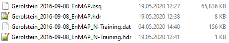
2. Unpack the data, remember the target folder. There should be two images in Envi format consisting of two files each (.bsq and .hdr, see image below).
3. Start the EnMAP-Box (please check the EnMAP-Box tutorials first if you don’t know how). You can close all pre-loaded data sources since they aren’t needed for this tutorial.
4. Add data sources Gerolstein_2016-09-08_EnMAP.bsq and Gerolstein_2016-09-08_EnMAP_N-Training.dat.

Use SIO tool

1. Open the SIO tool:

   1. If you don’t see the Processing Toolbox at the right part of the EnMAP-Box, activate it through View -> Panels -> Processing Toolbox
   2. In the Processing Toolbox navigate to EnMAP-Box -> Regression -> Spectral Index Optimizer.
   3. Double click to start.

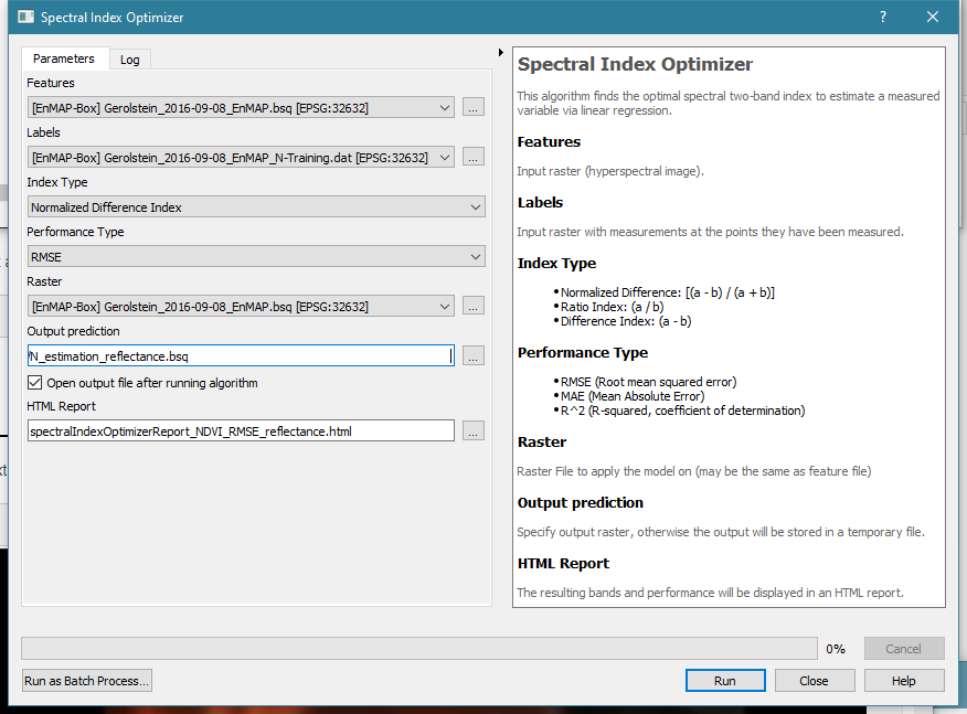
2. Use the SIO tool to create a map of N estimates:

   1. In the field Features, select Gerolstein_2016-09-08_EnMAP.bsq
   2. In the field Labels, select Gerolstein_2016-09-08_EnMAP_N-Training.dat
   3. You can select any Index Type and Performance Type you like.
   4. To save the N estimation in a file, click ... at the field Output prediction and enter a path and filename.
   5. Enter a filename for the HTML report or use the default filename.
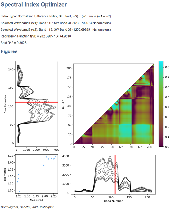
   6. Click Run to run the SIO tool.
   7. It should take only a few seconds, then the HTML report (see below) will open in your browser and the resulting N map will be available in the EnMAP-Box.

3. You can inspect the map in the EnMAP-Box viewer.

The SIO HTML report looks like this:

Calculate DASF and CSC

Broadleaf trees usually have higher leaf N concentrations and appear brighter than needleleaf trees. The brightness can be used to estimate N if both broadleaf and needleleaf trees are in your sample, but the correlation will be spurious (see DASF help text and Knyazikhin et al., 2013).

The Directional Area Scattering Factor (DASF) was invented to compensate for the brightness differences to estimate N from spectra without using the spurious correlation. So in the second part of this tutorial we will calculate the DASF of our image, use it to compensate brightness differences between broadleaf and needleleaf trees and estimate N with the resulting Canopy Scattering Coefficient (CSC) image.

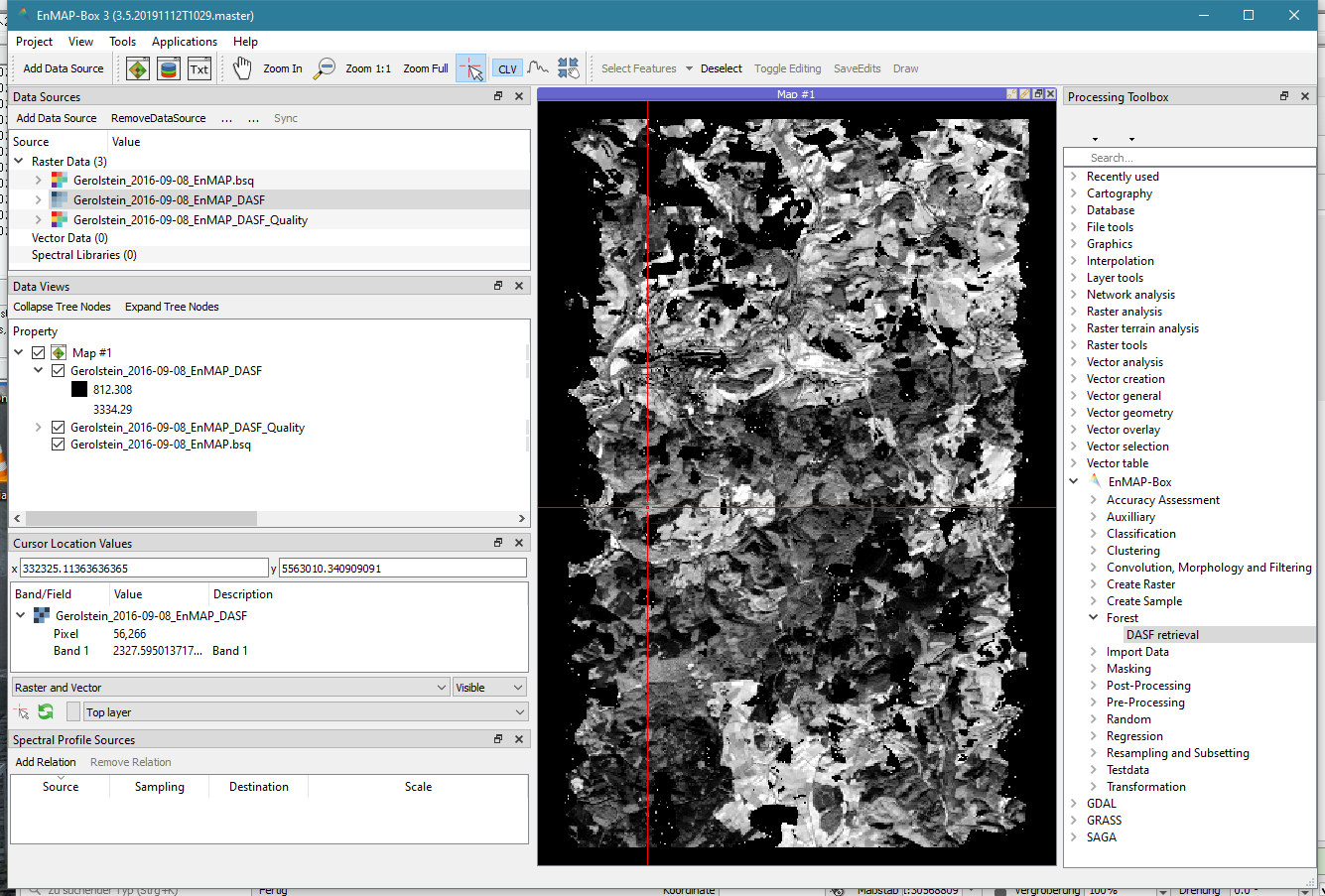
Calculate DASF

1. Open the DASF retrieval tool:

   1. In the Processing Toolbox navigate to EnMAP-Box -> Forest -> DASF retrieval
   2. Double click to start.

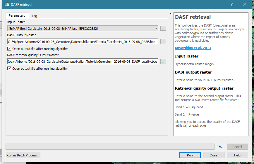
2. Select the hyperspectral reflectance image Gerolstein_2016-09-08_EnMAP.bsq as Input raster.

3. Specify output files for the DASF output raster and the quality output raster (optional).

4. Run the DASF retrieval tool. For the tutorial file it should only take about a minute.

The DASF is a single band image that is highly correlated to the bidirectional reflectance in the near infrared region of close forest pixels. Divide the hyperspectral reflectance image by the DASF to get the CSC. In the next step we will use the CSC to estimate N and compare the result to the estimation based on reflectance.

Calculate CSC

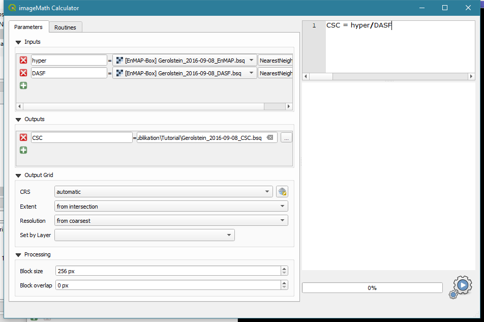
We will use the ImageMath application to divide the reflectance image by the DASF.

1. Open the ImageMath application: Navigate to Applications -> ImageMath
2. In the ImageMath Calculator we need to define input and output variables and an equation to create the output from the input.
3. In the grey field under “Inputs”, select the hyperspectral image and call it “hyper” in the white field at the left hand side.
4. Click on the green + to create a second input
5. Select the DASF and call it DASF
6. Under “Outputs”, select a filename for the CSC and call it CSC
7. Enter the equation “CSC = hyper/DASF” in the top right field. It uses the variable names we just defined in the Input and Output fields.
8. Start the calculation by clicking the gearwheel at the bottom right.

Estimate N using CSC

The Nitrogen concentration can be estimated from CSC analogous to the estimation from reflectance:

1. In the Processing Toolbox navigate to EnMAP-Box -> Regression -> Spectral Index Optimizer, double click to start.
2. In the field Features, select the CSC image.
3. In the field Labels, select Gerolstein_2016-09-08_EnMAP_N-Training.dat again.
4. You can select any Index Type and Performance Type you like.
5. To save the N estimation in a file, click ... at the field Output prediction and enter a path and filename.
6. Enter a filename for the HTML report or use the default filename.
7. click Run to run the SIO tool.

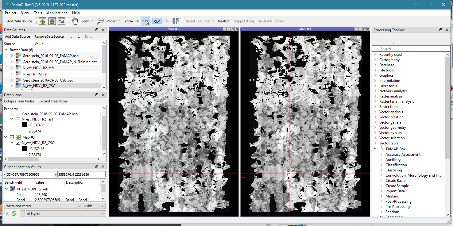
Discussion

Please use the results with caution.

Using the tutorial data, the correlograms will be nearly identical, no matter whether reflectance or CSC data is used. Consequently, the N maps will also be very similar (see image below). This may be different when different data sets are used.

The data set used for this tutorial is based on a field campaign with professional tree climbers who collected leaf samples. These samples were analysed in a laboratory. Unfortunately, only a very low number of samples can be used, because only few samples could be collected in the given time and some sampling points are located in gaps or areas with cloud shadows in the hyperspectral image. This limited data set does not allow for a reliable wall-to-wall estimation of N concentration.

In addition, the N estimation only makes sense for forest pixels, but the image contains many additional land use classes. Masking non-forest pixels is not part of the scope of this tutorial for now.

References

Knyazikhin, Y., Schull, M.A., Stenberg, P., Mõttus, M., Rautiainen, M., Yang, Y., Marshak, A., Latorre Carmona, P., Kaufmann, R.K., Lewis, P., Disney, M.I., Vanderbilt, V., Davis, A.B., Baret, F., Jacquemoud, S., Lyapustin, A. & Myneni, R.B. (2013). Hyperspectral remote sensing of foliar nitrogen content. Proceedings of the National Academy of Sciences, 110, E185-E192. DOI:10.1073/pnas.1210196109, http://www.pnas.org/content/110/3/E185.abstract